Bollinger Band based Backtest Strategy on S&P500
Executive
Summary
This report summarized my finding on above mentioned topic “Bollinger Band based Backtest Strategy on S&P500” as part of the learning process involved in Computational Investing Part 1 online course offered by Georgia Institute of Technology in Coursera. The whole backtest was done using Python 2.7 environment coupled with Eclipse Kepler IDE leveraging the power of numpy and panda dataframe structure. This report comprised of few parts. Part 1 will be a brief summary of the scope of this report. Part 2 will be a discussion of the suggested trading strategy and its backtest framework. Part 3 will touch more detail about performance assessment. As a conclusion of our report, this trading strategy has been proven to have some potential upside and flexibility to be tweaked depending on the financial climate and investors' risk tolerance level.
1. Scope of
Report
The scope of this report is to create a simple backtest framework based on Bollinger band. Particularly the report will outline discussion about portfolio selection (i.e. buy and sell signal), model and parameters discussion, its backtest framework, and performance assessment. In addition, the author will address some of the limitation faces and future work recommendation.
2. Model
discussion
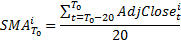
Before jump to the strategy itself, first we will discuss the definition of Bollinger band used throughout this report. By definition, Bollinger Band is a band constructed out of simple moving average. In order to construct the Bollinger Band, two volatility bands are placed above or below the simple moving average/rolling average curve. As far as this report was concerned, a lookback period of 20 working days are used in the calculation of simple moving average (SMA). Consequently the standard deviation plus the upper and lower band for stock(i) at any point of time (T0) were derived using the same lookback period and Bollinger std deviation multiplier of 2.
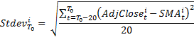


Similarly given any adjusted closing price of particular stock(i) at any point of time (T0), we could derived Bollinger multiplier (BM) which essentially the stdev multiplier by following expression

As per title of the report, the strategy will revolve around the usage of Bollinger Band as a technical indicator used to indicate a 'buy' or 'sell' signal. As benchmark index, we will be using S&P500 in our report. Consequently our stock selection came from S&P500 as well. In particular a basket of stocks listed under SP500 between period of 1st Jan 20008 and 31st Dec 2009 backtest period will all be considered as a potential 'buy' as long as following conditions were met
Buy
signal
1. T-1 (yesterday) stock BM ≥ yesterday stock BM threshold
2. T0 (today/trading day) stock BM ≤ today stock BM threshold
3. T0 (today/trading day) index/market BM ≥ 1
Sell
signal
As for the selling rule, we will be submitting a sell market order for the position at T+5 (5 days from the day we buy the stock) regardless whether profit or loss realized. There is no specific reason on why T+5 was chosen and this can be considered as one parameter involved in this strategy. Summarized in Figure 1 is the decision tree of this strategy.
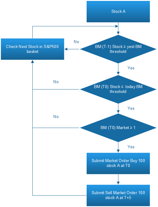
Figure 1 Buy and Sell signal decision tree illustration
The intuition here was to capitalize the benefit from buying stocks that underperform the market at trading day and selling it at a higher price 5 days later. With regards to volume of each trading, each trading consists of either buying or selling a quantity of 100 stocks of interest. To illustrate further with real example, following Figure 2 shows a series of buy and sell transaction with DeVry Education (DV) Group stock using today and yesterday BM threshold of -2 and market BM threshold of 1. Green vertical line indicates buy transaction while red vertical line indicates sell transaction.
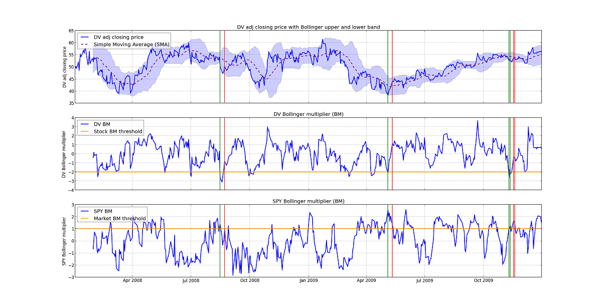
Figure 2 Illustration of buy and sell signal using DeVry Education Group (DV) stock
Different performance comparison under different input of two parameters (i.e. today and yesterday stock BM threshold) out of possible five parameters (i.e. today BM threshold, yesterday BM threshold, market BM threshold, stock holding period, backtest period) will be done as part of the sensitivity analysis and backtest framework.
3. Model Assessment
As per mentioned briefly in previous section, model assessment was done by tweaking two out of possible five parameters namely today stock BM and yesterday stock BM threshold. Specifically a sensitivity analysis ranging between -2 ≤ BM threshold ≤ -1 will be used in this report. The rest of three parameters were set at a fixed number. Market BM threshold was set to 1. Stock holding period before selling transaction was set to 5 days. Backtest period was 2 years period from 1st Jan 2008 to 31st Dec 2009.
The strategy's Sharpe ratio, as per shown in Figure 3, was in general inversely related to yesterday BM threshold level. Though both return and standard deviation of return went down, the overall reduction of Sharpe ratio was attributed more to reduction in return. Interestingly this seemed to contradict the original idea of capturing profit from buying stocks that seem to 'underperform' overall market. However taken into account our backtest period (i.e. year 2008-2009) which was the period when financial crisis occurred, one possible explanation was might due to a level of investors' risk tolerance. Another possible explanation was due to short holding period of 5 days which seems to be not enough for the position to be profitable.
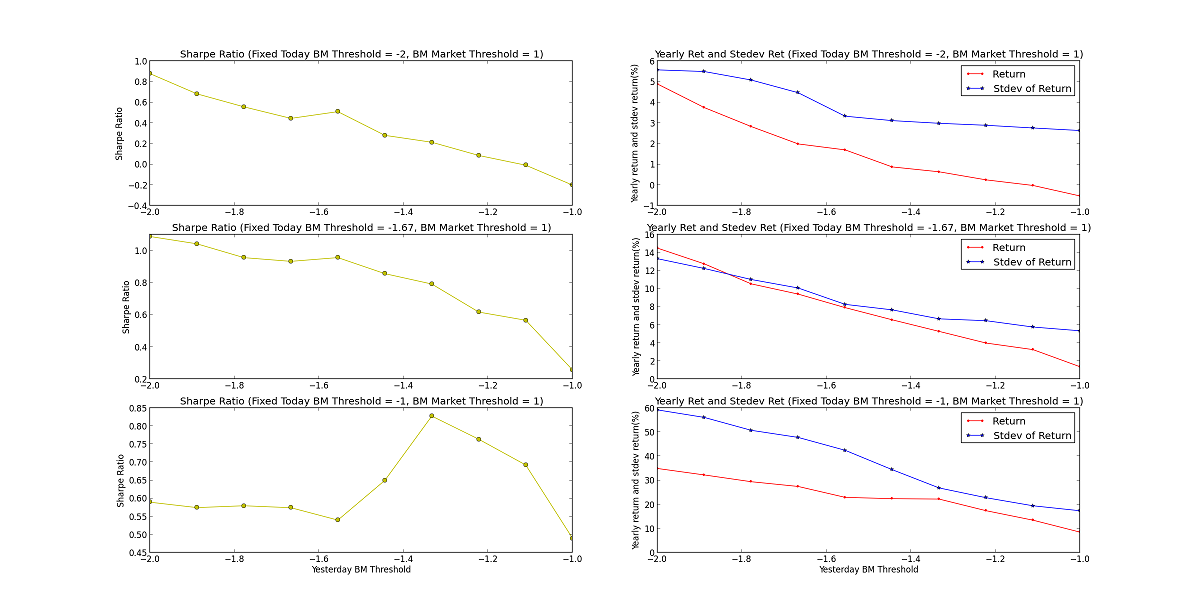
Figure 3 Sharpe ratio, return, and std deviation of return in
relation with varying yesterday BM threshold level
The relationship with respect to varying today BM threshold exhibited the cyclic relationship as shown in Figure 4 with observed peak for today BM threshold between -1.7 to -1.5. Given a backtest and holding period used in this report, momentum investing style appeared to be profitable as return outpaced the standard deviation within today BM threshold range of -1.7 to -1.5. To look for an optimal parameters, sensitivity analysis for both today and yesterday BM threshold was done. Result in Figure 5 showed the most optimal parameters within the range used in this report is for a combination of yesterday BM threshold within -2 to -1.7 and today BM threshold within -1.65 to -1.55. Overall highest Sharpe ratio obtained was around 1.10. Compared to a Sharpe ratio of -0.12 obtained by buying and holding an index, this strategy offered a reasonable performance across the different today and yesterday BM threshold combinations chosen.
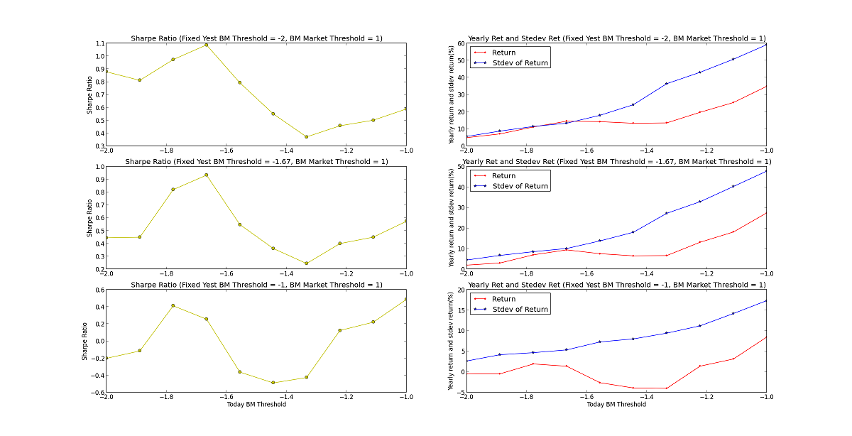
Figure 4 Sharpe ratio, return, and std deviation of return in relation with varying today BM threshold level
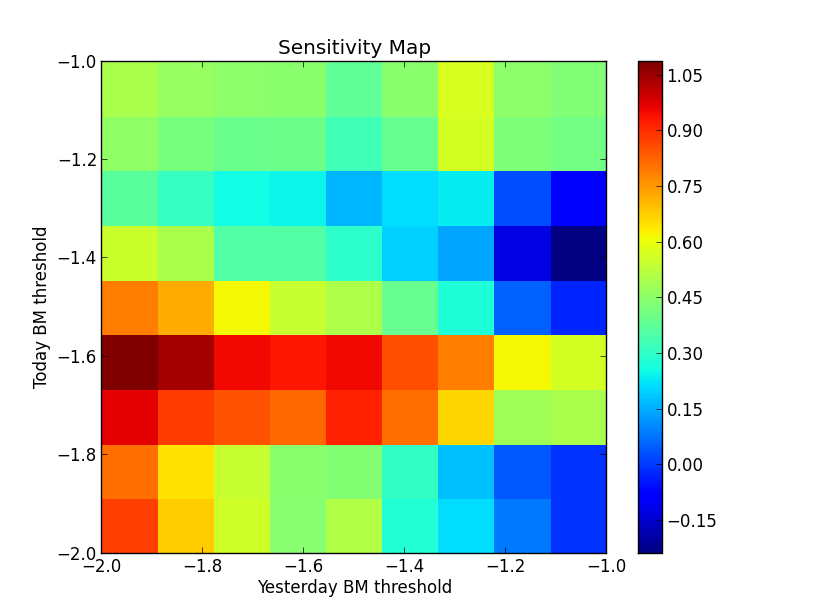
Figure 5 Sharpe Ratio sensitivity analysis by varying yesterday and today BM threshold level
4.
Conclusion & Future
Recommendation
In this report we have successfully developed a backtest framework utilizing Bollinger band as a buy or sell signal indicator. Particularly strategy performance under sensitivity analysis of two parameters namely yesterday and today stock Bollinger Multiplier (BM) was done. Rather than the original idea of buying “underperform” stocks, it appeared that performance was driven by some degree of price momentum within today BM threshold range of -1.7 to -1.5. Further given the backtest period used in this report, this strategy offered a reasonable performance with highest Sharpe ration of 1.10 as compared to -0.12 obtained by buying and holding the index. Further this strategy offered some level of flexibility as it was possible to explore five different parameters. For example in bull market it is wised to increase our holding period to gain more upside potential. However this statement needs further backtesting. Thus for future recommendation, the author would like to suggest to explore the remaining three different parameters (i.e. market BM threshold, stock holding period, and backtest period which involved different financial market scenario).